Boston House Prices#
Regression predictive modeling machine learning problem from end-to-end Python.
Tutorial from https://machinelearningmastery.com/machine-learning-with-python/
# 1. Prepare Problem
# a) Load libraries
import numpy
from numpy import arange
from matplotlib import pyplot
from pandas import read_csv
from pandas import set_option
from pandas.plotting import scatter_matrix
from sklearn.preprocessing import StandardScaler
from sklearn.model_selection import train_test_split
from sklearn.model_selection import KFold
from sklearn.model_selection import cross_val_score
from sklearn.model_selection import GridSearchCV
from sklearn.linear_model import LinearRegression
from sklearn.linear_model import Lasso
from sklearn.linear_model import ElasticNet
from sklearn.tree import DecisionTreeRegressor
from sklearn.neighbors import KNeighborsRegressor
from sklearn.svm import SVR
from sklearn.pipeline import Pipeline
from sklearn.ensemble import RandomForestRegressor
from sklearn.ensemble import GradientBoostingRegressor
from sklearn.ensemble import ExtraTreesRegressor
from sklearn.ensemble import AdaBoostRegressor
from sklearn.metrics import mean_squared_error
# b) Load dataset
filename = 'datasets/housing.csv'
names = ['CRIM', 'ZN', 'INDUS', 'CHAS', 'NOX', 'RM', 'AGE', 'DIS', 'RAD', 'TAX', 'PTRATIO', 'B', 'LSTAT', 'MEDV']
dataset = read_csv(filename, names=names, delim_whitespace=True)
print(dataset)
        CRIM    ZN  INDUS  CHAS    NOX     RM   AGE     DIS  RAD    TAX  \
0    0.00632  18.0   2.31     0  0.538  6.575  65.2  4.0900    1  296.0
1    0.02731   0.0   7.07     0  0.469  6.421  78.9  4.9671    2  242.0
2    0.02729   0.0   7.07     0  0.469  7.185  61.1  4.9671    2  242.0
3    0.03237   0.0   2.18     0  0.458  6.998  45.8  6.0622    3  222.0
4    0.06905   0.0   2.18     0  0.458  7.147  54.2  6.0622    3  222.0
..       ...   ...    ...   ...    ...    ...   ...     ...  ...    ...
501  0.06263   0.0  11.93     0  0.573  6.593  69.1  2.4786    1  273.0
502  0.04527   0.0  11.93     0  0.573  6.120  76.7  2.2875    1  273.0
503  0.06076   0.0  11.93     0  0.573  6.976  91.0  2.1675    1  273.0
504  0.10959   0.0  11.93     0  0.573  6.794  89.3  2.3889    1  273.0
505  0.04741   0.0  11.93     0  0.573  6.030  80.8  2.5050    1  273.0

     PTRATIO       B  LSTAT  MEDV
0       15.3  396.90   4.98  24.0
1       17.8  396.90   9.14  21.6
2       17.8  392.83   4.03  34.7
3       18.7  394.63   2.94  33.4
4       18.7  396.90   5.33  36.2
..       ...     ...    ...   ...
501     21.0  391.99   9.67  22.4
502     21.0  396.90   9.08  20.6
503     21.0  396.90   5.64  23.9
504     21.0  393.45   6.48  22.0
505     21.0  396.90   7.88  11.9

[506 rows x 14 columns]
/var/folders/kf/_5f4g2zd40n8t2rnn343psmc0000gn/T/ipykernel_84223/2592008294.py:4: FutureWarning: The 'delim_whitespace' keyword in pd.read_csv is deprecated and will be removed in a future version. Use ``sep='\s+'`` instead
  dataset = read_csv(filename, names=names, delim_whitespace=True)
print(dataset.dtypes)
CRIM       float64
ZN         float64
INDUS      float64
CHAS         int64
NOX        float64
RM         float64
AGE        float64
DIS        float64
RAD          int64
TAX        float64
PTRATIO    float64
B          float64
LSTAT      float64
MEDV       float64
dtype: object
# 2. Summarize Data
# a) Descriptive statistics

description = dataset.describe()
print(description)
             CRIM          ZN       INDUS        CHAS         NOX          RM  \
count  506.000000  506.000000  506.000000  506.000000  506.000000  506.000000
mean     3.613524   11.363636   11.136779    0.069170    0.554695    6.284634
std      8.601545   23.322453    6.860353    0.253994    0.115878    0.702617
min      0.006320    0.000000    0.460000    0.000000    0.385000    3.561000
25%      0.082045    0.000000    5.190000    0.000000    0.449000    5.885500
50%      0.256510    0.000000    9.690000    0.000000    0.538000    6.208500
75%      3.677083   12.500000   18.100000    0.000000    0.624000    6.623500
max     88.976200  100.000000   27.740000    1.000000    0.871000    8.780000

              AGE         DIS         RAD         TAX     PTRATIO           B  \
count  506.000000  506.000000  506.000000  506.000000  506.000000  506.000000
mean    68.574901    3.795043    9.549407  408.237154   18.455534  356.674032
std     28.148861    2.105710    8.707259  168.537116    2.164946   91.294864
min      2.900000    1.129600    1.000000  187.000000   12.600000    0.320000
25%     45.025000    2.100175    4.000000  279.000000   17.400000  375.377500
50%     77.500000    3.207450    5.000000  330.000000   19.050000  391.440000
75%     94.075000    5.188425   24.000000  666.000000   20.200000  396.225000
max    100.000000   12.126500   24.000000  711.000000   22.000000  396.900000

            LSTAT        MEDV
count  506.000000  506.000000
mean    12.653063   22.532806
std      7.141062    9.197104
min      1.730000    5.000000
25%      6.950000   17.025000
50%     11.360000   21.200000
75%     16.955000   25.000000
max     37.970000   50.000000
correlation = dataset.corr()
print(correlation)
             CRIM        ZN     INDUS      CHAS       NOX        RM       AGE  \
CRIM     1.000000 -0.200469  0.406583 -0.055892  0.420972 -0.219247  0.352734
ZN      -0.200469  1.000000 -0.533828 -0.042697 -0.516604  0.311991 -0.569537
INDUS    0.406583 -0.533828  1.000000  0.062938  0.763651 -0.391676  0.644779
CHAS    -0.055892 -0.042697  0.062938  1.000000  0.091203  0.091251  0.086518
NOX      0.420972 -0.516604  0.763651  0.091203  1.000000 -0.302188  0.731470
RM      -0.219247  0.311991 -0.391676  0.091251 -0.302188  1.000000 -0.240265
AGE      0.352734 -0.569537  0.644779  0.086518  0.731470 -0.240265  1.000000
DIS     -0.379670  0.664408 -0.708027 -0.099176 -0.769230  0.205246 -0.747881
RAD      0.625505 -0.311948  0.595129 -0.007368  0.611441 -0.209847  0.456022
TAX      0.582764 -0.314563  0.720760 -0.035587  0.668023 -0.292048  0.506456
PTRATIO  0.289946 -0.391679  0.383248 -0.121515  0.188933 -0.355501  0.261515
B       -0.385064  0.175520 -0.356977  0.048788 -0.380051  0.128069 -0.273534
LSTAT    0.455621 -0.412995  0.603800 -0.053929  0.590879 -0.613808  0.602339
MEDV    -0.388305  0.360445 -0.483725  0.175260 -0.427321  0.695360 -0.376955

              DIS       RAD       TAX   PTRATIO         B     LSTAT      MEDV
CRIM    -0.379670  0.625505  0.582764  0.289946 -0.385064  0.455621 -0.388305
ZN       0.664408 -0.311948 -0.314563 -0.391679  0.175520 -0.412995  0.360445
INDUS   -0.708027  0.595129  0.720760  0.383248 -0.356977  0.603800 -0.483725
CHAS    -0.099176 -0.007368 -0.035587 -0.121515  0.048788 -0.053929  0.175260
NOX     -0.769230  0.611441  0.668023  0.188933 -0.380051  0.590879 -0.427321
RM       0.205246 -0.209847 -0.292048 -0.355501  0.128069 -0.613808  0.695360
AGE     -0.747881  0.456022  0.506456  0.261515 -0.273534  0.602339 -0.376955
DIS      1.000000 -0.494588 -0.534432 -0.232471  0.291512 -0.496996  0.249929
RAD     -0.494588  1.000000  0.910228  0.464741 -0.444413  0.488676 -0.381626
TAX     -0.534432  0.910228  1.000000  0.460853 -0.441808  0.543993 -0.468536
PTRATIO -0.232471  0.464741  0.460853  1.000000 -0.177383  0.374044 -0.507787
B        0.291512 -0.444413 -0.441808 -0.177383  1.000000 -0.366087  0.333461
LSTAT   -0.496996  0.488676  0.543993  0.374044 -0.366087  1.000000 -0.737663
MEDV     0.249929 -0.381626 -0.468536 -0.507787  0.333461 -0.737663  1.000000
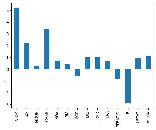
skew = dataset.skew()
skew.plot(kind='bar')
pyplot.show()
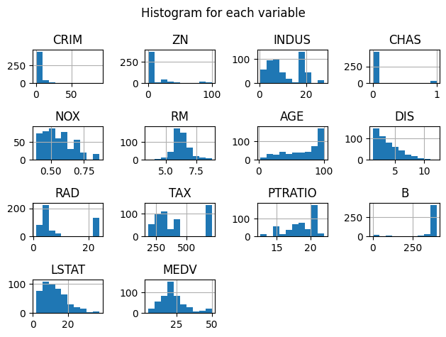
# 2) Data Visualization
# a) Univariate Plots
fig = pyplot.figure(figsize=(12, 8))
dataset.hist(sharex=False, sharey=False)
pyplot.suptitle('Histogram for each variable')
pyplot.tight_layout()
pyplot.show()
<Figure size 1200x800 with 0 Axes>
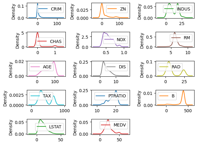
dataset.plot(kind='density', subplots=True, layout=(5,3), sharex=False, sharey=False)
pyplot.tight_layout()
pyplot.show()
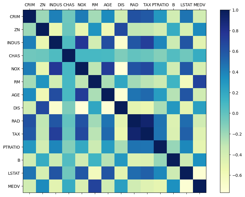
names = ['CRIM', 'ZN', 'INDUS', 'CHAS', 'NOX', 'RM', 'AGE', 'DIS', 'RAD', 'TAX', 'PTRATIO', 'B', 'LSTAT', 'MEDV']
correlation_matrix = dataset.corr()
fig = pyplot.figure(figsize=(12, 8))
ax = fig.add_subplot(111)
cax = ax.matshow(correlation_matrix, cmap='YlGnBu')
fig.colorbar(cax)

ticks = numpy.arange(0, 14, 1)
ax.set_xticks(ticks)
ax.set_yticks(ticks)
ax.set_xticklabels(names)
ax.set_yticklabels(names)

pyplot.show()
# 3. Prepare Data
# a) Data Cleaning
# b) Feature Selection

array = dataset.values
X = array[:, 0:13]
Y = array[:, 13]

validation_size = 0.20
seed = 7
X_train, X_validation, Y_train, Y_validation = train_test_split(X, Y, test_size=validation_size, random_state=seed)

num_folds = 10
seed = 7
scoring = 'neg_mean_squared_error'

# 4. Evaluate Algorithms
# a) Split-out validation dataset
# b) Test options and evaluation metric
# c) Spot Check Algorithms

models = []
models.append(('LR', LinearRegression()))
models.append(('LASSO', Lasso()))
models.append(('EN', ElasticNet()))
models.append(('KNN', KNeighborsRegressor()))
models.append(('CART', DecisionTreeRegressor()))
models.append(('SVR', SVR()))

results = []
names = []

for name, model in models:
    kfold = KFold(n_splits=num_folds, random_state=seed, shuffle=True)
    cv_results = cross_val_score(model, X_train, Y_train, cv=kfold, scoring=scoring)
    results.append(cv_results)
    names.append(name)
    msg = "%s: %f (%f)" % (name, cv_results.mean(), cv_results.std())
    print(msg)
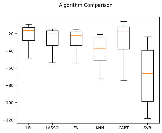
LR: -22.006009 (12.188886)
LASSO: -27.105803 (13.165915)
EN: -27.923014 (13.156405)
KNN: -39.808936 (16.507968)
CART: -26.532459 (19.752973)
SVR: -67.824695 (32.801531)
# d) Compare Algorithms

fig = pyplot.figure()
fig.suptitle('Algorithm Comparison')
ax = fig.add_subplot(111)
pyplot.boxplot(results)
ax.set_xticklabels(names)
pyplot.show()
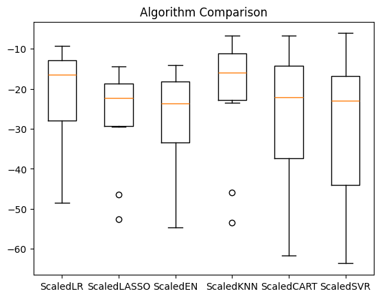
# 5. Improve Accuracy

# a) Data Transformation

pipelines = []
pipelines.append(('ScaledLR', Pipeline([('Scaler', StandardScaler()), ('LR', LinearRegression())])))
pipelines.append(('ScaledLASSO', Pipeline([('Scaler', StandardScaler()), ('LASSO', Lasso())])))
pipelines.append(('ScaledEN', Pipeline([('Scaler', StandardScaler()), ('EN', ElasticNet())])))
pipelines.append(('ScaledKNN', Pipeline([('Scaler', StandardScaler()), ('KNN', KNeighborsRegressor())])))
pipelines.append(('ScaledCART', Pipeline([('Scaler', StandardScaler()), ('CART', DecisionTreeRegressor())])))
pipelines.append(('ScaledSVR', Pipeline([('Scaler', StandardScaler()), ('SVR', SVR())])))

results = []
names = []

for name, model in pipelines:
    kfold = KFold(n_splits=num_folds, random_state=seed, shuffle=True)
    cv_results = cross_val_score(model, X_train, Y_train, cv=kfold, scoring=scoring)
    results.append(cv_results)
    names.append(name)
    msg = "%s: %f (%f)" % (name, cv_results.mean(), cv_results.std())
    print(msg)
ScaledLR: -22.006009 (12.188886)
ScaledLASSO: -27.205896 (12.124418)
ScaledEN: -28.301160 (13.609110)
ScaledKNN: -21.456867 (15.016218)
ScaledCART: -27.845546 (18.620515)
ScaledSVR: -29.570404 (18.052973)
pyplot.boxplot(results, labels=names)
pyplot.title('Algorithm Comparison')
pyplot.show()
/var/folders/kf/_5f4g2zd40n8t2rnn343psmc0000gn/T/ipykernel_84223/1115231628.py:1: MatplotlibDeprecationWarning: The 'labels' parameter of boxplot() has been renamed 'tick_labels' since Matplotlib 3.9; support for the old name will be dropped in 3.11.
  pyplot.boxplot(results, labels=names)
# improve results with tuning

scaler = StandardScaler().fit(X_train)
rescaledX = scaler.transform(X_train)

k_values = numpy.array([1,3,5,7,9, 11, 13, 15, 17, 19, 21])
param_grid = dict(n_neighbors=k_values)
model = KNeighborsRegressor()
kfold = KFold(n_splits=num_folds, random_state=seed, shuffle=True)
grid = GridSearchCV(estimator=model, param_grid=param_grid, scoring=scoring, cv=kfold)
grid_result = grid.fit(rescaledX, Y_train)
print("Best: %f using %s" % (grid_result.best_score_, grid_result.best_params_))
Best: -19.497829 using {'n_neighbors': 1}
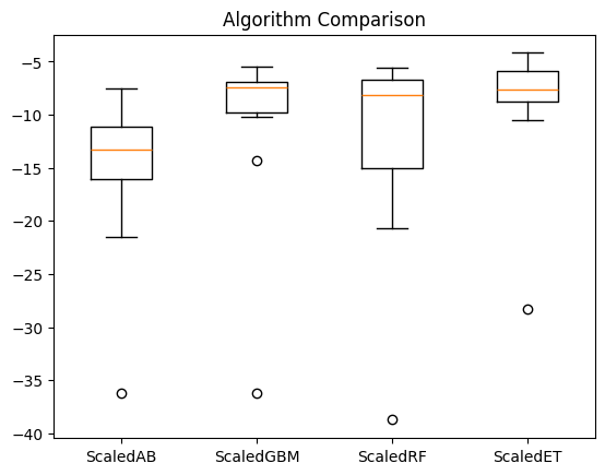
# ensembles

ensembles = []

ensembles.append(('ScaledAB',  Pipeline([('Scaler', StandardScaler()), ('AB', AdaBoostRegressor())])))
ensembles.append(('ScaledGBM', Pipeline([('Scaler', StandardScaler()), ('GBM', GradientBoostingRegressor())])))
ensembles.append(('ScaledRF', Pipeline([('Scaler', StandardScaler()), ('RF', RandomForestRegressor())])))
ensembles.append(('ScaledET', Pipeline([('Scaler', StandardScaler()), ('ET', ExtraTreesRegressor())])))

results = []
names = []

for name, model in ensembles:
    kfold = KFold(n_splits=num_folds, random_state=seed, shuffle=True)
    cv_results = cross_val_score(model, X_train, Y_train, cv=kfold, scoring=scoring)
    results.append(cv_results)
    names.append(name)
    msg = "%s: %f (%f)" % (name, cv_results.mean(), cv_results.std())
    print(msg)
ScaledAB: -15.618859 (7.759029)
ScaledGBM: -11.011864 (8.717405)
ScaledRF: -12.711214 (9.897574)
ScaledET: -9.312014 (6.577605)
pyplot.boxplot(results, labels=names)
pyplot.title('Algorithm Comparison')
pyplot.show()
/var/folders/kf/_5f4g2zd40n8t2rnn343psmc0000gn/T/ipykernel_84223/2660017936.py:1: MatplotlibDeprecationWarning: The 'labels' parameter of boxplot() has been renamed 'tick_labels' since Matplotlib 3.9; support for the old name will be dropped in 3.11.
  pyplot.boxplot(results, labels=names)
# tune ensemble methods
scaler = StandardScaler().fit(X_train)
rescaledX = scaler.transform(X_train)
param_grid = dict(n_estimators=numpy.array([50, 100, 150, 200, 250, 300, 350, 400, 450, 500]))
model = GradientBoostingRegressor(random_state=seed)
kfold = KFold(n_splits=num_folds, random_state=seed, shuffle=True)
grid = GridSearchCV(estimator=model, param_grid=param_grid, scoring=scoring, cv=kfold)
grid_result = grid.fit(rescaledX, Y_train)
print("Best: %f using %s" % (grid_result.best_score_, grid_result.best_params_))
Best: -10.522386 using {'n_estimators': 450}
# final model

# prepare the model
scaler = StandardScaler().fit(X_train)
rescaledX = scaler.transform(X_train)
model = GradientBoostingRegressor(random_state=seed, n_estimators=450)
model.fit(rescaledX, Y_train)

# transform the validation dataset
rescaledX_validation = scaler.transform(X_validation)
predictions = model.predict(rescaledX_validation)
print(mean_squared_error(Y_validation, predictions))
11.955246016638654